Glossary

PROPHET StatGuide: Glossary

Taken from http://www.basic.northwestern.edu/statguidefiles/sg_glos.html

For the one-sample t test, the null hypothesis is that the population mean equals a specific value. For a two-sided test, the alternative hypothesis is that the mean does not equal that value. It is also possible to have a one-sided test with the alternative hypothesis that the mean is greater than the specified value, if it is theoretically impossible for the mean to be less than the specified value. One could alternatively perform one-sided test with the alternative hypothesis that the mean is less than the specified value, if it were theoretically impossible for the mean to be greater than the specified value.

One-sided tests usually have more power than two-sided tests, but they require more stringent assumptions. They should only be used when those assumptions (such as the mean always being at least as large as they specified value for the one-sample t test) apply.

between effects:

In a repeated measures ANOVA, there will be at least one factor that is measured at each level for every subject. This is a within (repeated measures) factor. For example, in an experiment in which each subject performs the same task twice, trial (or trial number) is a within factor. There may also be one or more factors that are measured at only one level for each subject, such as gender. This type of factor is a between or grouping factor.

bias:

An estimator for a parameter is unbiased if its expected value is the true value of the parameter. Otherwise, the estimator is biased.

binary variable:

A binary random variable is a discrete random variable that has only two possible values, such as whether a subject dies (event) or lives (non-event). Such events are often described as success vs failure.

boxplot:

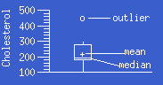
A boxplot is a graph summarizing the distribution of a set of data values. The upper and lower ends of of the center box indicate the 75th and 25th percentiles of the data, the center box indicates the median, and the center + indicates the mean. Suspected outliers appear in a boxplot as individual points o or x outside the box. The o outlier values are known as outside values, and the x outlier values as far outside values.

If the difference (distance) between the 75th and 25th percentiles of the data is H, then the outside values are those values that are more than 1.5H but no more than 3H above the upper quartile, and those values that are more than 1.5H but no more than 3H below the lower quartile. The far outside values are values that are at least 3H above the upper quartile or 3H below the lower quartile.

Examples of these plots illustrate various situations.

cell:

In a multi-factor ANOVA or in a contingency table, a cell is an individual combination of possible levels (values) of the factors. For example, if there are two factors, gender with values male and female and risk with values low, medium, and high, then there are 6 cells: males with low risk, males with medium risk, males with high risk, females with low risk, females with medium risk, and females with high risk.

censoring:

In an experiment in which subjects are followed over time until an event of interest (such as death or other type of failure) occurs, it is not always possible to follow every subject until the event is observed. Subjects may drop out of the study and be lost to follow-up, or be deliberately withdrawn, or the end of the data collection period may arrive before the event is observed to happen. For such a subject, all that is known is that the time to the event was at least as long as the time to when the subject was last observed. The observed time to the event under such circumstances is censored. Survival analysis methods generally allow for censored data. Censoring may occur from the right (observation stops before the event is observed), as in censorship for survival analysis, or from the left (observation does not begin until after the event has occurred).

central tendency:

The generalized concept of the "average" value of a distribution. Typical measures of central tendency are the mean, the median, the mode, and the geometric mean.

centroid:

The centroid of a set of multi-dimensional data points is the data point that is the mean of the values in each dimension. For X-Y data, the centroid is the point at (mean of the X values, mean of the Y values). A simple linear regression line always passes through the centroid of the X-Y data.

chi-square test for goodness of fit:

The chi-square test for goodness of fit tests the hypothesis that the distribution of the population from which nominal data are drawn agrees with a posited distribution. The chi-square goodness-of-fit test compares observed and expected frequencies (counts). The chi-square test statistic is basically the sum of the squares of the differences between the observed and expected frequencies, with each squared difference divided by the corresponding expected frequency.

chi-square test for independence (Pearson's):

Pearson's chi-square test for independence for a contingency table tests the null hypothesis that the row classification factor and the column classification factor are independent. Like the chi-square goodness-of-fit test, the chi-square test for independence compares observed and expected frequencies (counts). The expected frequencies are calculated by assuming the null hypothesis is true. The chi-square test statistic is basically the sum of the squares of the differences between the observed and expected frequencies, with each squared difference divided by the corresponding expected frequency. Note that the chi-square statistic is always calculated using the counted frequencies. It can not be calculated using the observed proportions, unless the total number of subjects (and thus the frequencies) is also known.

conservative:

A hypothesis test is conservative if the actual significance level for the test is smaller than the stated significance level of the test. An example is the Kolmogorov-Smirnov distribution test, which becomes conservative when the parameters of the distribution are estimated from the data instead of being specified in advance. A conservative test may incorrectly fail to reject the null hypothesis, and thus is less powerful than was expected.

consistent:

A hypothesis test is consistent for a specified alternative hypothesis if the power of the test for the alternative hypothesis approaches 1 as the sample size becomes infinitely large.

contaminated normal distribution:

A contaminated normal distribution is a type of mixture distribution for which observed values can come from one of multiple normal distributions. For example, in taking measurements of blood pressure from a population, the distribution for males may be a normal distribution, the distribution for females may also be a normal distribution, but if the two normal distributions do not have the same mean and variance, then the composite distribution is not normal.

A common type of contaminated normal distribution is a composite of two normal distributions with the same mean, but with different variances, such that only a minority of the values come from the distribution with the larger variance. Such a distribution is heavy-tailed relative to the normal distribution. If the proportion of values from the distribution with the larger variance is small enough, the contaminated normal distribution may look like a normal distribution with outliers. In such a situation, one should be alert to the possibility of a connection or common trait among the outlying values that might suggest that all come from a second distribution with a different variance.

contingency table:

If individual values are cross-classified by levels in two different attributes (factors), such as gender and tumor vs no tumor, then a contingency table is the tabulated counts for each combination of levels of the two factors, with the levels of one factor labeling the rows of the table, and the levels of the other factor labeling the columns of the table. For the factors gender and presence of tumor, each with two levels, we would get a 2x2 contingency table, with rows Male and Female, and columns Tumor and No Tumor.

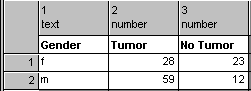
The counts for each cell in the table would be the number of subjects with the corresponding row level of gender and column level of tumor vs no tumor: females with tumors in row 1, column 1; females without tumors in row 1, column 2; males with tumors in row 2, column 1; and males without tumors in row 2, column 2, as shown in the picture. Contingency tables are also known as cross-tabulations. The most common method of analyzing such tables statistically is to perform a (Pearson) chi-square test for independence or Fisher's exact test.

correlation:

Correlation is the linear association between two random variables X and Y. It is usually measured by a correlation coefficient, such as Pearson's r, such that the value of the coefficient ranges from -1 to 1. A positive value of r means that the association is positive; i.e., that if X increases, the value of Y tends to increase linearly, and if X decreases, the value of Y tends to decrease linearly. A negative value of r means that the association is negative; i.e., that if X increases, the value of Y tends to decrease linearly, and if X decreases, the value of Y tends to increase linearly. The larger r is in absolute value, the stronger the linear association between X and Y. If r is 0, X and Y are said to be uncorrelated, with no linear association between X and Y. Independent variables are always uncorrelated, but uncorrelated variables need not be independent.

covariate:

A covariate is a variable that may affect the relationship between two variables of interest, but is not of intrinsic interest itself. As in blocking or stratification, a covariate is often used to control for variation that is not attributable to the variables under study. A covariate may be a discrete factor, like a block effect, or it may be a continuous variable, like the X variable in an analysis of covariance.

Note that some people use the term covariate to include all the variables that may effect the response variable, including both the primary (predictor) variables, and the secondary variables we call covariates.

curvilinear functions:

A curvilinear function is one whose value, when plotted, will follow a continuous but not necessarily straight line, such as a polynomial, logistic, exponential, or sinusoidal curve.

death density function:

The death density function is a time to failure function that gives the instantaneous probability of the event (failure). That is, in a survival experiment where the event is death, the value of the density function at time T is the probability that a subject will die precisely at time T. This differs from the hazard function, which gives the probability conditional on a subject having survived to time T. The death density function is always nonnegative (greater than or equal to 0), and a peak in the function indicates a time at which the probability of failure is high.

Other names for the death density function are probability density function and unconditional failure rate. Related functions are the hazard function, the conditional instantaneous probability of the event (failure) given survival up to that time; and the survival function, which represents the probability that the event (failure) has not yet occurred. The cumulative hazard function is the integral over time of the hazard function, and is estimated as the negative logarithm of the survival function.

distribution function:

A distribution function (also known as the probability distribution function) of a continuous random variable X is a mathematical relation that gives for each number x, the probability that the value of X is less than or equal to x. For example, a distribution function of height gives, for each possible value of height, the probability that the height is less than or equal to that value. For discrete random variables, the distribution function is often given as the probability associated with each possible discrete value of the random variable; for instance, the distribution function for a fair coin is that the probability of heads is 0.5 and the probability of tails is 0.5.

distribution-free tests:

Distribution-free tests are tests whose validity under the null hypothesis does not require a specification of the population distribution(s) from which the data have been sampled.

expected cell frequencies:

For nominal (categorical) data in which the count of items in each category has been tabulated, the observed frequency is the actual count, and the expected frequency is the count predicted by the theoretical distribution underlying the data. For example, if the hypothesis is that a certain plant has yellow flowers 3/4 of the time and white flowers 1/4 of the time, then for 100 plants, the expected frequencies will be 75 for yellow and 25 for white. The observed frequencies will be the actual counts for 100 plants (say, 73 and 27).

factors:

A factor is a single discrete classification scheme for data, such that each item classified belongs to exactly one class (level) for that classification scheme. For example, in a drug experiment involving rats, sex (with levels male and female) or drug received could be factors. A one-way analysis of variance involves a single factor classifying the subjects (e.g., drug received); multi-factor analysis of variance involves multiple factors classifying the subjects (e.g., sex and drug received).

fixed effects:

In an experiment using a fixed-effect design, the results of the experiment apply only to the populations included in the experiment. Those populations include all (or at least most of) those of interest. This is true for many experiments, where the effects are due to such variables as gender, age categories, disease states, or treatments. When the populations included in the experiment are a random subset of those of interest, then the experiment follows a random-effects design.

Multiple comparisons tests for an analysis of variance may be applied when the effects are fixed. They are not appropriate if the effects are random.

Whether an effect is considered random or fixed may depend on the circumstances. A factory may conduct an experiment comparing the output of several machines. If those machines are the only ones of interest (because they constitute the entire set of machines owned by that company), then machine will be a fixed effect. If the machines were instead selected randomly from among those owned by the company, then machine would be a random effect.

Fisher's exact test:

Fisher's exact test for a 2x2 contingency table is a test of the null hypothesis that the row classification factor and the column classification factor are independent. Fisher's exact test consists of calculating the actual (hypergeometric) probability of the observed 2x2 contingency table with respect to all other possible 2x2 contingency tables with the same column and row totals. The probabilities of all such tables that are each no more likely than the observed table are calculated. The sum of these probabilities is the P value. If the sum is less than or equal to the specified significance level, then the null hypothesis is rejected.

goodness of fit:

Goodness-of-fit tests test the conformity of the observed data's empirical distribution function with a posited theoretical distribution function. The chi-square goodness-of-fit test does this by comparing observed and expected frequency counts. The Kolmogorov-Smirnov test does this by calculating the maximum vertical distance between the empirical and posited distribution functions.

hazard function:

The hazard function is a time to failure function that gives the instantaneous probability of the event (failure) given that it has not yet occurred. That is, in a survival experiment where the event is death, the value of the hazard function at time T is the probability that a subject will die precisely at time T, given that the subject has survived to time T. The function may increase with time, meaning that the longer subjects survive, the more likely it becomes that they will die shortly (as for cancer patients who do not respond to treatment). It may decrease with time, meaning that the longer subjects survive, the more likely it is that they will survive into the near future (as for post-operative survival for gunshot victims). It may remain constant, as for a population with a (negative) exponential survival distribution. Or it may have a more complicated shape, like the well-known "bathtub" curve for human mortality, where the hazard is high for newborns, drops quickly, stays low through adulthood, and then rises again in old age.

Other names for the hazard function are instantaneous failure rate, force of mortality, conditional mortality rate, and age-specific failure rate. Related functions are the death density function, the unconditional instantaneous probability of the event (failure); and the survival function, which represents the probability that the event (failure) has not yet occurred. The cumulative hazard function is the integral over time of the hazard function, and is estimated as the negative logarithm of the survival function.

heavy-tailed:

A heavy-tailed distribution is one in which the extreme portion of the distribution (the part farthest away from the median) spreads out further relative to the width of the center (middle 50%) of the distribution than is the case for the normal distribution. For a symmetric heavy-tailed distribution like the Cauchy distribution, the probability of observing a value far from the median in either direction is greater than it would be for the normal distribution. Boxplots may help in detecting heavy-tailedness; normal probability plots may also help in detecting heavy-tailedness.

histogram:

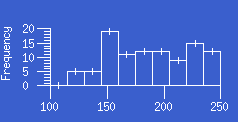
A histogram is a graph of grouped (binned) data in which the number of values in each bin is represented by the area of a rectangular box.

homoscedasticity (homogeneity of variance):

Normal-theory-based tests for the equality of population means such as the t test and analysis of variance, assume that the data come from populations that have the same variance, even if the test rejects the null hypothesis of equality of population means. If this assumption of homogeneity of variance is not met, the statistical test results may not be valid. Heteroscedasticity refers to lack of homogeneity of variances.

(in)appropriate use of chi-square test:

Pearson's chi-square test for independence for a contingency table involves using a normal approximation to the actual distribution of the frequencies in the contingency table. This approximation becomes less reliable when the expected frequencies for the contingency table are very small. A standard (and conservative) rule of thumb (due to Cochran) is to avoid using the chi-square test for contingency tables with expected cell frequencies less than 1, or when more than 20% of the contingency table cells have expected cell frequencies less than 5. In such cases, an alternate test like Fisher's exact test for a 2x2 contingency table should be considered for a more accurate evaluation of the data.

independent:

Two random variables are independent if their joint probability density is the product of their individual (marginal) probability densities. Less technically, if two random variables A and B are independent, then the probability of any given value of A is unchanged by knowledge of the value of B. A sample of mutually independent random variables is an independent sample.

index plot:

An index plot of data values is a plot of each value (Y) against its order in the data set (X). If data are entered into a table in the order in which they are collected, for example, then a plot of data value against row number will produce an index plot. An index plot may help detect correlation between successive data values, a sign of lack of independence.

interaction:

In multi-factor analysis of variance, factors A and B interact if the effect of factor A is not independent of the level of factor B. For example, in an drug experiment involving rats, there would be an interaction between the factors sex and treatment if the effect of treatment was not the same for males and females.

kurtosis:

Kurtosis is a measure of the heaviness of the tails in a distribution, relative to the normal distribution. A distribution with negative kurtosis (such as the uniform distribution) is light-tailed relative to the normal distribution, while a distribution with positive kurtosis (such as the Cauchy distribution) is heavy-tailed relative to the normal distribution.

levels within factors:

When a factor is used to classify subjects, each subject is assigned to one class value; e.g., male or female for the factor sex or the specific treatment given for the factor treatment. These individual class values within a factor are called levels. Each subject is assigned to exactly one level for each factor.

Each unique combination of levels for each factor is a cell.

leverage:

Leverage is a measure of the amount of influence a given data value has on a fitted linear regression. For a change in an observed Y value, the leverage is the proportional change in the fitted Y value.

life table method:

For survival studies, life tables are constructed by partitioning time into intervals (usually equal intervals), and then counting for each time interval: the number of subjects alive at the start of the interval, the number who die during the interval, and the number who are lost to follow-up or withdrawn during the interval. Those lost or withdrawn are censored. Those alive at the end of a time interval were at risk for the entire interval. Under the usual actuarial method of survival function estimation for life tables, the estimate of the probability of survival within each time interval is calculated by assuming that any values censored in that interval were at risk for half the interval. Death can be replaced by any other identifiable event. Unlike the Kaplan-Meier product-limit method, the life table survival estimate can still be calculated even if the exact survival or censoring times are not known for each individual, as long as the number of individuals who die or are censored within each time interval is known.

light-tailed:

A light-tailed distribution is one in which the extreme portion of the distribution (the part farthest away from the median) spreads out less far relative to the width of the center (middle 50%) of the distribution than is the case for the normal distribution. For a symmetric light-tailed distribution like the uniform distribution, the probability of observing a value far from the median in either direction is smaller than it would be for the normal distribution. Boxplots may help in detecting light-tailedness; normal probability plots may also help in detecting light-tailedness.

linear functions:

A linear function of one or more X variables is a linear combination of the values of the variables:
Y = b0 + b1*X1 + b2*X2 + ... + bk*Xk.
An X variable in the equation could be a curvilinear function of an observed variable (e.g., one might measure distance, but think of distance squared as an X variable in the model, or X2 might be the square of X1), as long as the overall function (Y) remains a sum of terms that are each an X variable multiplied by a coefficient (i.e., the function Y is linear in the coefficients). Sometimes, an apparently nonlinear function can be made linear by a transformation of Y, such as the function
Y = exp(b0 + b1*X1),
which can be made a linear function by taking the logarithm of Y
(log(Y) = b0 + b1*X1),
and then considering log(Y) to be the overall function.

linear logistic model:

A linear logistic model assumes that for each possible set of values for the independent (X) variables, there is a probability p that an event (success) occurs. Then the model is that Y is a linear combination of the values of the X variables:
Y = b0 + b1*X1 + b2*X2 + ... + bk*Xk,
where Y is the logit tranformation of the probability p.

linear regression:

In a linear regression, the fitted (predicted) value of the response variable Y is a linear combination of the values of one or more predictor (X) variables:
fitted Y = b0 + b1*X1 + b2*X2 + ... + bk*Xk.
An X variable in the model equation could be a nonlinear function of an observed variable (e.g., one might observe distance, but use distance squared as an X variable in the model, or X2 might be the square of X1), as long as the fitted Y remains a sum of terms that are each an X variable multiplied by a coefficient. The most basic linear regression model is simple linear regression, which involves one X variable:
fitted Y = b0 + b1*X.
Multiple linear regression refers to a linear regression with more than one X variable.

location:

The generalized concept of the "average" value of a distribution. Typical measures of location are the mean, the median, the mode, and the geometric mean.

logit transformation:

The logit transformation Y of a probabilty p of an event is the logarithm of the ratio between the probability that the event occurs and the probability that the event does not occur:
Y = log(p/(1-p)).

log-rank test:

In survival analysis, a log-rank test compares the equality of k survival functions by creating a sequence of kx2 contingency tables (k survival functions by event observed/event not observed at that time) one at each (uncensored) observed event time, and calculating a statistic based on the observed and expected values for these contingency tables. This test is also known as the Mantel-Cox (Mantel-Haenszel) test. The Tarone-Ware and Gehan-Breslow tests are weighted variants of the log-rank test; the Peto and Peto log-rank test involves a different generalization of this log-rank scheme.

matched samples:

Matching, also known as pairing (with two samples) and blocking (with multiple samples) involves matching up individuals in the samples so as to minimize their dissimilarity except in the factor(s) under study. For example, in pre-test/post-test studies, each subject is paired (matched) with himself, so that the difference between the pre-test and post-test responses can be attributed to the change caused by taking the test, and not to differences between the individuals taking the test. A study involving animals might be blocked by matching up animals from the same litter or from the same cage. The goal is to minimize the variation within the pairs or blocks while maximizing the variation between them. This will minimize variation between subjects that is not attributable to the factors under study by attributing it to the blocking factor. The matched items in a pair or in a block are related by their membership in that pair or block. Other methods for controlling for variation between subjects for variables that are not of direct interest are stratification and the use of covariates.

method of maximum likelihood:

The method of maximum likelihood is a general method of finding estimated (fitted) values of parameters. Estimates are found such that the joint likelihood function, the product of the values of the distribution function for each observed data value, is as large as possible. The estimation process involves considering the observed data values as constants and the parameter to be estimated as a variable, and then using differentiation to find the value of the parameter that maximizes the likelihood function.

The maximum likelihood method works best for large samples, where it tends to produce estimators with the smallest possible variance. The maximum likelihood estimators are often biased in small samples.

The maximum likelihood estimates for the slope and intercept in simple linear regression, are the same as the least squares estimates when the underlying distribution for Y is normal. In this case, the maximum likelihood estimators are thus unbiased. In general, however, the maximum likelihood and least squares estimates need not be the same.

measures of association:

For cross-tabulated data in a contingency table, a measure of association measures the degree of association between the row and column classification variables. Measures of association include the coefficient of contingency, Cramer's V, Kendall's tau-B, Kendall's tau-C, gamma, and Spearman's rho,

method of least squares:

The method of least squares is a general method of finding estimated (fitted) values of parameters. Estimates are found such that the sum of the squared differences between the fitted values and the corresponding observed values is as small as possible. In the case of simple linear regression, this means placing the fitted line such that the sum of the squares vertical distances between the observed points and the fitted line is minimized.

median:

The median of a distribution is the value X such that the probability of an observation from the distribution being below X is the same as the probability of the observation being above X. For a continuous distribution, this is the same as the value X such that the probability of an observation being less than or equal to X is 0.5.

median remaining lifetime:

For survival studies using life tables, the median remaining lifetime for an interval of the life table is the estimate of the additional elapsed time before only half the individuals alive at the beginning of current interval are still alive. This is also known as the median residual lifetime.

mixed models:

Factors in an analysis of variance (ANOVA) may be either fixed or random. Multi-factor ANOVA models in which at least one effect is fixed and at least one effect is random are called mixed models, especially a two-factor factorial ANOVA in which one factor is fixed and the other is random. A randomized block ANOVA is also usually a mixed model, since the factor of interest is usually a fixed effect.

For two-factor factorial ANOVA, a mixed model is also referred to as a Type III model. (If both effects are fixed, it's a Type I model, and if both effects are random, it's a Type II model.)

Sometimes, the term mixed model is also applied to ANOVA models in which at least one factor is a repeated measures (within) factor, and at least one factor is a grouping (between) factor.

mixture distribution:

A mixture distribution is a distribution for which observed values can come from one of multiple distributions. For example, in taking measurements of blood pressure from a population, the distribution for males may be a normal distribution, the distribution for females may also be a normal distribution, but if the two normal distributions do not have the same mean and variance, then the composite distribution is not normal.

multicollinearity:

In a multiple regression with more than one X variable, two or more X variables are collinear if they are nearly linear combinations of each other. Multicollinearity can make the calculations required for the regression unstable, or even impossible. It can also produce unexpectedly large estimated standard errors for the coefficients of the X variables involved. Multicollinearity is also known as collinearity and ill conditioning.

multiple comparisons:

An analysis of variance F test for a specific factor tests the hypothesis that all the level means are the same for that factor. However, if the null hypothesis is rejected, the F test does not give information as to which level means differ from which other level means. Multiplicity issues make doing individual tests to compare each pair of means inappropriate unless the nominal (comparisonwise) significance level is adjusted to account for the number of pairs (as in a Bonferroni method). An alternative approach is to devise a test (such as Tukey's test) specifically designed to keep the overall (experimentwise) significance level at the desired value while allowing for the comparison of all possible pairs of means. This is a multiple comparisons test.

multiple regression:

Multiple regression refers to a regression model in which the fitted value of the response variable Y is a function of the values of one or more predictor (X) variables. The most common form of multiple regression is multiple linear regression, a linear regression model with more than one X variable.

multiplicity of testing:

Even when the null hypothesis is true, a statistical hypothesis test has a small probability (the preselected alpha-level or significance level) of falsely rejecting the null hypothesis. With a significance level of 0.05, this could be considered as the probability of seeing 20 come up on a 20-sided fair die. If multiple tests are done (the die is rolled multiple times), even if the null hypothesis in each case is true, the probability of getting at least one such false rejection (seeing 20 turn up at least once) increases. For the common problem of comparing pairwise mean differences following an analysis of variance, the probability of seeing at least one such false rejection could approach 90% when there are 10 level means in the factor. To avoid the multiplicity problem, multiple comparison tests have been devised to allow for simultaneous inference about all the pairwise comparisons while maintaining the desired significance level.

multi-sample problem:

In the multi-sample problem, multiple independent random samples are collected, and then the samples are used to test a hypothesis about the populations from which the samples came (e.g., whether the means of the populations are all identical).

nonlinear functions:

A nonlinear function is one that is not a linear function, and can not be made into a linear function by transforming the Y variable.

nonlinear regression:

In a nonlinear regression, the fitted (predicted) value of the response variable is a nonlinear function of one or more X variables.

nonparametric tests:

Nonparametric tests are tests that do not make distributional assumptions, particularly the usual distributional assumptions of the normal-theory based tests. These include tests that do not involve population parameters at all (truly nonparametric tests such as the chi-square goodness of fit test), and distribution-free tests, whose validity does not depend on the population distribution(s) from which the data have been sampled. In particular, nonparametric tests usually drop the assumption that the data come from normally distributed populations. However, distribution-free tests generally do make some assumptions, such as equality of population variances.

normal (Gaussian) distribution:

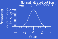
The normal or Gaussian distribution is a continuous symmetric distribution that follows the familiar bell-shaped curve. The distribution is uniquely determined by its mean and variance. It has been noted empirically that many measurement variables have distributions that are at least approximately normal. Even when a distribution is nonnormal, the distribution of the mean of many independent observations from the same distribution becomes arbitrarily close to a normal distribution as the number of observations grows large. Many frequently used statistical tests make the assumption that the data come from a normal distribution.

normal probability plot:

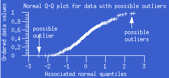
A normal probability plot, also known as a normal Q-Q plot or normal quantile-quantile plot, is the plot of the ordered data values (as Y) against the associated quantiles of the normal distribution (as X). For data from a normal distribution, the points of the plot should lie close to a straight line. Examples of these plots illustrate various situations.

null hypothesis:

The null hypothesis for a statistical test is the assumption that the test uses for calculating the probability of observing a result at least as extreme as the one that occurs in the data at hand. For the two-sample unpaired t test, the null hypothesis is that the two population means are equal, and the t test involves finding the probability of observing a t statistic at least as extreme as the one calculated from the data, assuming the null hypothesis is true.

one-sample problem:

In the one-sample problem, an independent random sample is collected, and then that sample is used to test a hypothesis about the population from which the sample came (e.g., whether the mean of the population is 0, or any other fixed constant chosen in advance). Paired samples are usually reduced to a one-sample problem by replacing each pair of responses by the difference between them (e.g., in a pre-test/post-test experiment, recording the change from pre-test to post-test).

order statistics:

If the data values in a sample are sorted into increasing order, then the ith order statistic is the ith largest data value. For a sample of size N, common order statistics are the extremes, the minimum (first order statistic) and maximum (Nth order statistic). Quantiles or percentiles such as the median are also calculated from order statistics.

outliers:

Outliers are anomalous values in the data. They may be due to recording errors, which may be correctable, or they may be due to the sample not being entirely from the same population. Apparent outliers may also be due to the values being from the same, but nonnormal (in particular, heavy-tailed), population distribution.

P value:

In a statistical hypothesis test, the P value is the probability of observing a test statistic at least as extreme as the value actually observed, assuming that the null hypothesis is true. This probability is then compared to the pre-selected significance level of the test. If the P value is smaller than the significance level, the null hypothesis is rejected, and the test result is termed significant.

The P value depends on both the null hypothesis and the alternative hypothesis. In particular, a test with a one-sided alternative hypothesis will generally have a lower P value (and thus be more likely to be significant) than a test with a two-sided alternative hypothesis. However, one-sided tests require more stringent assumptions than two-sided tests. They should only be used when those assumptions apply.

paired samples:

Pairing involves matching up individuals in two samples so as to minimize their dissimilarity except in the factor under study. For example, in pre-test/post-test studies, each subject is paired (matched) with himself, so that the difference between the pre-test and post-test responses can be attributed to the change caused by taking the test, and not to differences between the individuals taking the test. Such data are analyzed by examining the paired differences.

parallelism assumption:

For analysis of covariance (ANCOVA), it is assumed that the populations can each be correctly modeled by a straight-line simple linear regression. The parallelism assumption is that the regressions all have the same slope. The assumption can be tested by a test of equality for slopes. If the assumption of equality of slopes does not hold, then a subsequent test of equality of intercepts (elevations) is meaningless, since it requires that the slopes be equal.

pooled estimate of the variance:

The pooled estimate of the variance is a weighted average of each individual sample's variance estimate. When the estimates are all estimates of the same variance (i.e., when the population variances are equal), then the pooled estimate is more accurate than any of the the individual estimates.

population:

The population is the universe of all the objects from which a sample could be drawn for an experiment. If a representative random sample is chosen, the results of the experiment should be generalizable to the population from which the sample was drawn, but not necessarily to a larger population. For example, the results of medical studies on males may not be generalizable for females.

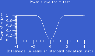
power:

The power of a test is the probability of (correctly) rejecting the null hypothesis when it is in fact false. The power depends on the significance level (alpha-level) of the test, the components of the calculation of the test statistic, and on the specific alternative hypothesis under consideration. For the two-sample unpaired t test, an alternative hypothesis would be that the difference between the two population means was some specific non-zero value, such as 1.5; the components of the test statistic include the sample sizes, sample means, and sample variances. The greater the power of a two-sample unpaired t test, the better able it is to correctly reject (i.e., declare significant) small but real differences between the two population means. A power curve plots the power against the actual difference between the population means.

product-limit method:

For survival studies, the product-limit (Kaplan-Meier) estimate of survival is calculated by dividing time into intervals such that each interval ends at the time of an observation, whether censored or uncensored. The probability of survival is calculated at the end of each interval, with censored observations assumed to have occurred just after uncensored ones. The product-limit survival function is a step function that changes value at each time point associated with an uncensored value.

qualitative:

Qualitative variables are variables for which an attribute or classification is measured. Examples of qualitative variables are gender or disease state.

quantitative:

Quantitative variables are variables for which a numeric value representing an amount is measured.

random effects:

When the populations included in an experiment are a random subset of those of interest, then the experiment follows a random-effects design. In a experiment using a random-effects design, the results of the experiment apply not only to the populations included in the experiment, but to the wider set of populations from which the subset was taken. For example, subjects in a repeated measures (within factors) design are considered a random effect because we are interested not in the particular subjects chosen for the experiment, but the entire population of potential subjects. Similarly, blocks are often a random effect in analysis of variance.

Multiple comparisons tests for an analysis of variance are not applied when the effects are random.

Whether an effect is to considered random or fixed may depend on the circumstances. A factory may conduct an experiment comparing the output of several machines. If those machines are the only ones of interest (because they constitute the entire set of machines owned by that company), then machine will be a fixed effect. If the machines were instead selected randomly from among those owned by the company, then machine would be a random effect.

random sample:

A random sample of size N is a collection of N objects that are independent and identically distributed. In a random sample, each member of the population has an equal chance of becoming part of the sample.

random variable:

A random variable is a rule that assigns a value to each possible outcome of an experiment. For example, if an experiment involves measuring the height of people, then each person who could be a subject of the experiment has associated value, his or her height. A random variable may be discrete (the possible outcomes are finite, as in tossing a coin) or continuous (the values can take any possible value along a range, as in height measurements).

randomized block design:

A randomized block analysis of variance design such as one-way blocked ANOVA is created by first grouping the experimental subjects into blocks such that the subjects in each block are as similar as possible (e.g., littermates), and there are as many subjects in each block as there are levels of the factor of interest, and then randomly assigning a different level of the factor to each member of the block, such that each level occurs once and only once per block. The blocks are assumed not to interact with the factor.

rank tests:

Rank tests are nonparametric tests that are calculated by replacing the data by their rank values. Rank tests may also be applied when the only data available are relative rankings. Examples of rank tests include the Wilcoxon signed rank test, the Mann-Whitney rank sum test, the Kruskal-Wallis test, and Friedman's test.

repeated measures ANOVA:

In a repeated measures ANOVA, there will be at least one factor that is measured at each level for every subject in the experiement. This is a within (repeated measures) factor. For example, in an experiment in which each subject performs the same task twice is a repeated measures design, with trial (or trial number) as the within factor. If every subject performed the same task twice under each of two conditions, for a total of 4 observations for each subject, then both trial and condition would be within factors.

In a repeated measures design, there may also be one or more factors that are measured at only one level for each subject, such as gender. This type of factor is a between or grouping factor.

residuals:

A residual is the difference between the observed value of a response measurement and the value that is fitted under the hypothesized model. For example, in a two-sample unpaired t test, the fitted value for a measurement is the mean of the sample from which it came, so the residual would be the observed value minus the sample mean.

resistant:

A statistic is resistant if its value does not change substantially when an arbitrary change, no matter how large, is made in any small part of the data. For example, the median is a resistant measure of location, while the mean is not; the mean can be drastically affected by making a single data value arbitrarily large, whereas the median can not.

robust:

Robust statistical tests are tests that operate well across a wide variety of distributions. A test can be robust for validity, meaning that it provides P values close to the true ones in the presence of (slight) departures from its assumptions. It may also be robust for efficiency, meaning that it maintains its statistical power (the probability that a true violation of the null hypothesis will be detected by the test) in the presence of those departures.

scale:

The generalized concept of the variability or dispersion of a distribution. Typical measures of scale are variance, standard deviation, range, and interquartile range.

Scale and spread both refer to the same general concept of variability.

shape:

The general form of a distribution, often characterized by its skewness and kurtosis (heavy or light tails relative to a normal distribution).

significance level:

The significance level (also known as the alpha-level) of a statistical test is the pre-selected probability of (incorrectly) rejecting the null hypothesis when it is in fact true. Usually a small value such as 0.05 is chosen. If the P value calculated for a statistical is smaller than the significance level, the null hypothesis is rejected.

skewness:

Skewness is a lack of symmetry in a distribution. Data from a positively skewed (skewed to the right) distribution have values that are bunched together below the mean, but have a long tail above the mean. (Distributions that are forced to be positive, such as annual income, tend to be skewed to the right.) Data from a negatively skewed (skewed to the left) distribution have values that are bunched together above the mean, but have a long tail below the mean. Boxplots may be useful in detecting skewness to the right or to the left; normal probabilty plots may also be useful in detecting skewness to the right or to the left.

spread:

The generalized concept of the variability of a distribution. Typical measures of spread are variance, standard deviation, range, and interquartile range.

Spread and scale both refer to the same general concept of variability.

stratification:

Stratification involves dividing a sample into homogeneous subsamples based on one or more characteristics of the population. For example, samples may be stratified by 10-year age groups, so that, for example, all subjects aged 20 to 29 are in the same age stratum in each group. Like blocking or the use of covariates, stratification is often used to control for variation that is not attributable to the variables under study. Stratification can be done on data that has already been collected, whereas blocking is usually done by matching subjects before the data are collected. Potential disadvantages to stratification are that the number of subjects in a given stratum may not be uniform across the groups being studied, and that there may be only a small number of subjects in a particular stratum for a particular group.

structural zeros:

The process that creates the observations that appear in a contingency table may produce cells in the contingency table in which observations can never occur. The zero values that must occur in these cells are structural zeroes. For example, a contingency table of cancer incidence by sex and type of cancer must have the value 0 in the cell for males and ovarian cancer, but the expected number of males with ovarian cancer will not be 0 as long as there is are at least 1 male and 1 ovarian cancer patient among the observations. A contingency table containing one or more structural zeroes is an incomplete table. Pearson's chi-square test for independence and Fisher's exact test are not designed for contingency tables with structural zeroes.

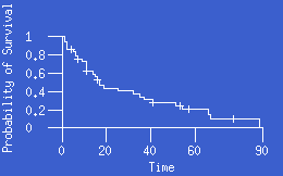
survival function:

The survival function is a time to failure function that gives the probability that an individual survives (does not experience an event) past a given time. That is, in a survival experiment where the event is death, the value of the survival function at time T is the probability that a subject will die at some time greater than T. The survival function always has a value between 0 and 1 inclusive, and is nonincreasing. The function is used to find percentiles for survival time, and to compare the survival experience of two or more groups.

The mortality function is simply 1 minus the survival function. Other names for the survival function are survivorship function and cumulative survival rate. Related functions are the hazard function, the conditional instantaneous probability of the event (failure) given survival up to that time; and the death density function, which represents the unconditional probability that the event occurs exactly at time t. Steeper survival curves (faster drop off toward 0) suggest larger values for the hazard or death density functions, and shorter survival times. The cumulative hazard function is the integral over time of the hazard function, and is estimated as the negative logarithm of the survival function.

test of independence:

A test of independence for a contingency table tests the null hypothesis that the row classification factor and the column classification factor are independent. Two such tests are Pearson's chi-square test for independence and Fisher's exact test.

time to failure distributions:

In survival analysis, data is collected on the time until an event is observed (or censoring occurs). Often this event is associated with a failure (such as death or cessation of function). The probability distribution of such times can be represented by different functions. Three of these are: the survival function, which represents the probability that the event (failure) has not yet occurred; the death density function, which is the instantaneous probability of the event (failure); and the hazard function, which is the instantaneous probability of the event (failure) given that it has not yet occurred. The cumulative hazard function is the integral over time of the hazard function, and is estimated as the negative logarithm of the survival function.

transformation:

A transformation of data values is done by applying the same function to each data value, such as by taking logarithms of the data.

truncated distribution:

A distribution is truncated if observed values must fall within a restricted range, instead of the expected range over all possible real values. For example, a observation from a normal distribution can take any real value between -infinity and +infinity. An observation from a truncated normal distribution might only take on values greater than 0, or less than 2.

two-sample problem:

In the two-sample problem, two independent random samples are collected, and then the samples are used to test a hypothesis about the populations from which the samples came (e.g., whether the means of the two populations are identical).

two-way layout:

The two-way layout refers to a two-way classification in which there are two factors affecting the observed response measurements. Each possible combination of levels from both factors is observed, usually once each. The interaction between the two factors is generally assumed to be 0. The randomized block design is one example of a two-way layout.

violation of assumptions:

Statistical hypothesis tests generally make assumptions about the population(s) from which the data were sampled. For example, many normal-theory-based tests such as the t test and ANOVA assume that the data are sampled from one or more normal distributions, as well as that the variances of the different populations are the same (homoscedasticity:). If test assumptions are violated, the test results may not be valid.

Welch-Satterthwaite t test:

The Welch-Satterthwaite t test is an alternative to the pooled-variance t test, and is used when the assumption that the two populations have equal variances seems unreasonable. It provides a t statistic that asymptotically (that is, as the sample sizes become large) approaches a t distribution, allowing for an approximate t test to be calculated when the population variances are not equal.

within effects:

In a repeated measures ANOVA, there will be at least one factor that is measured at each level for every subject. This is a within (repeated measures) factor. For example, in an experiment in which each subject performs the same task twice, trial number is a within factor. There may also be one or more factors that are measured at only one level for each subject, such as gender. This type of factor is a between or grouping factor.

Peace and survival of life on Earth as we know it are threatened by human activities that lack a commitment to humanitarian values. Destruction of nature and natural resources results from ignorance, greed, and a lack of respect for the Earth's living things... . It is not difficult to forgive destruction in the past, which resulted from ignorance. Today, however, we have access to more information, and it is essential that we re-examine ethically what we have inherited, what we are responsible for, and what we will pass on to coming generations. Clearly this is a pivotal generation... . Our marvels of science and technology are matched if not outweighed by many current tragedies, including human starvation in some parts of the world, and extinction of other life forms... . We have the capability and responsibility. We must act before it is too late. Tenzin Gyatso the fourteenth Dalai Lama.